3-Dimensional Two-Points Correlation Function for Comparing Biological Fiber Networks

Ⅰ. Introduction

One purpose of tissue engineering is to develop hybrid tissue constructs that replace either a part of or the whole biological tissue. To offer support and shape, these hybrid tissue constructs often consist of cells embedded in fibrillar scaffolds that are made of micron-sized polymeric fibers.

In tissue engineering, a biofactor (e.g., cells, genes, and proteins) is implanted into a porous degradable material called a scaffold. Scaffolds play an important role in tissue regeneration by preserving tissue volume, delivering biofactors, and providing temporary mechanical function [1]. Various materials (e.g., ceramic and polymers), especially polymers, have been used for tissue scaffolds. Polymers have been largely used for scaffold materials due to their excellent processing properties [2]. Fibrillar polymeric scaffolds, which are made of micron-sized polymeric fibers, have received widespread attention as versatile extracellular matrix-like materials that have induced a synthesis of tissues and organs, or cell carriers. These provide the structural support for cell attachment and subsequent tissue development.

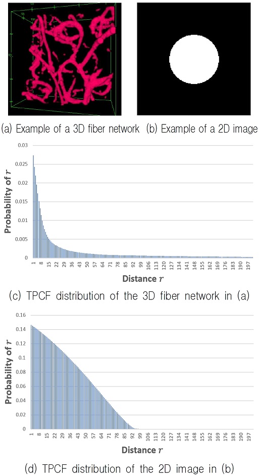
Apparently, the polymeric fibers form a network which naturally exists as a 3-dimensional structure. Recognizing the level of complexity in a biological fiber network is one way to improve the quality of a hybrid tissue construct. In this paper, we propose a new method to simplify the characteristics of a 3-dimensional biological fiber network onto a 2-dimensional. This will allow us to compare any two 3D biological fiber networks in an easier way. Specifically, our study utilizes this method in order to compare the complexities between biological networks (see the Fig. 3(a) for example) formed by poly-ε-capro-lactone (PCL) fibers having diameters within the 5-20 µm range.

Ⅱ. Related Works

There have been previous several research studies that have compared biological networks by developing a parameter. Recently, Maria et al. [3] suggested several parameters based on a minimum spanning tree (MST) to determine the level of randomness (or regularity) of a child brain network. Extreme topologies of MSTs have a star-like tree on one end and a line-like tree on the other end. One specific parameter developed by them is a tree hierarchy parameter. Physically, the parameter has the purpose of balancing the reduction of longest paths between all nodes and overload prevention. The value of the parameter lies between 0 and 1. If the brain network is a line-like topology network, the value approaches 0. If the brain network is a star-like topology, the value approaches 0.5.

Centrality analysis is also useful for analyzing biological networks and helps us to understand the underlying biological process. For instance, Newman listed several different types of centralities in his survey [4]: degree centrality, eigenvector centrality, Katz centrality, closeness centrality and betweenness centrality. In degree centrality, an important node is involved in a large number of interactions. Physically, this centrality indicates how well a node is connected in terms of direct connections. This parameter can be seen as an index of the node's communication activity.

In eigenvector centrality, a node is central if it has many central neighbors. Katz centrality, a general case of the degree centrality measures the number of all nodes that can be connected through a path while the contributions of distant nodes are penalized. In closeness centrality, an important node is typically close to, and can communicate quickly with, other nodes. It is based on proximity and measures how easily a node can reach other nodes in a network. Thus, it represents the measure of independence or efficiency of the node. Physically, it measures the mean distance from a node to other nodes. Finally, betweenness centrality of a node refers the number of paths passing through the node. Betweenness centrality represents how important a node is in terms of connecting to other nodes. So, it is useful as an index of the potential of a node control over communication. Physically, it is the number of geodesic paths passing through a specific node.

Newman also proposed a ‘local clustering parameter’. This parameter, physically, indicates the average probability that a pair of a node u’s neighbors are neighbors to each other. In relation to the local clustering, the concept of a ‘structural hole’ deserve attention. The structural hole refers to the missing links between neighbors (we actually expect that those links exist). If the local clustering has a low value, it is believed that there exist many number of structural holes.

Aside from studies focusing on biological networks, there are several research studies in the literature on scale-free social networks. For example, Butts [5][6] discussed ‘covariance’ as well as ‘structural distance’ parameters based on the adjacent matrix. These parameters assume that the networks have the same size. Physically, the graph covariance is simply the covariance of the two adjacent matrices, taken as a collection of edge variables. We can compute the correlation with the covariance. Physically, this correlation parameter means that the existence of a specific edge between node u and node v is compared between adjacency matrices.

Regarding Two-point correlation function (TPCF), several properties of N-point probability functions were examined by Frisch et al. [7] and Torquator et al. [8]. R. Ridgway et al. [9] used a 2-dimensional TPCF in order to segment a mice placenta. F.Janoos et al. [10] improved the computation cost and the achieved high precision of segmentation on a 2D TPCF feature space. L. Cooper et al. [11] developed a new fast and deterministic method for 2D TPCF calculations.

Since the bilogical network exists natually in a 3-dimesinal space, we need to extend 2D TPCF to 3D TPCF.

In the following section 3, we will discuss our proposed method and describe how we developed 3-dimensional TPCF. Section 4 will present the results of our approach and a future direction.

III. Method

3.2 3-dimensional TPCF

$$ S_2^{\left(FG\right)}\left(r\right)$$ characterizes the fiber structure in our experimental fiber network data. $$ S_2^{\left(FG\right)}\left(r\right)$$ is the probability of the endpoints of the line segment landing on FG after repeatedly throwing a line segment of length r within the 3D fiber network. Hence, the distribution of $$ S_2^{\left(FG\right)}\left(r\right)$$ depending on the value r represents the number of times that two points are correlated with each other in a given 3D fiber network.

In order to express $$ S_2^{\left(FG\right)}\left(r\right)$$ in a mathematical form, we need an indicator function of the form of Iⁱ(x,w) where x is a voxel in a given image and ω is the realization of a fiber network. The indicator function is defined as:

$\[ I^i\left(x,\omega \right)=\{\begin{array}{c}1, x\in 0\\ 0, x\notin 0\end{array} , \]$

(1)

In a 3D image of size, l×m×n, $$ S_2^{\left(FG\right)}\left(r\right)$$ can be calculated using an indicator autocorrelation C^(BG) which is defined as follows:

$\[ \begin{array}{c}{C}^{\left(FG\right)}\left(∆x,∆y,∆z\right)=\hfill \\ \sum _l^{}\sum _m^{}\sum _n^{}{I}^{\left(FG\right)}\left(l,m,n\right)I^{\left(FG\right)}\left(l+∆x,m+∆y,n+∆z\right)\hfill \end{array} \]$

(2)

where Δx,Δy,Δz∈Ƶ. Next, we normalize C^FG to calculate the probabilities. The normalized autocorrelation with $$ {\widehat{C}}^{FG}$$ is calculated as follows:

$\[ {\widehat{C}}^{\left(FG\right)}=C^{\left(FG\right)}{/}^e\left(1_{L\times M\times N}\text{*}{1}_{L\times M\times N}\right) \]$

(3)

where 1_L×M×N is the L×M×N matrix filled with 1, /^e represnts an elementwise division, and * represents convolution.

Then, isotropic TPCF $$ S_2^{\left(FG\right)}\left(r\right)$$ can be calculated as:

$\[ \begin{array}{c}{S}_2^{\left(FG\right)}\left(r\right)=\frac{∆\varphi }{\pi }\frac{∆\theta }{2\pi }\sum _{k_1=0}^{\frac{2\pi }{∆\theta }-1}\sum _{k_2=\frac{\pi }{2}}^{\frac{\pi }{2}+\frac{\pi }{∆\varphi }-1} \hfill \\ {\widehat{C}}^{\left(FG\right)}\left(rcos\left(k_1∆\theta \right)\text{sin}\left(k_2∆\varphi \right),rsin\left(k_1∆\theta \right)\text{sin}\left(k_2∆\varphi \right),rcos\left(k_2∆\varphi \right)\right)\hfill \end{array} \]$

(4)

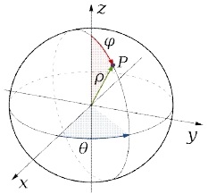
where Δθ and Δϕ are angular intervals as shown in the following Fig. 1. By using the Eq. (4) we can sample the points of the autocorrelation matrix radially on a southern hemisphere of the Fig. 1.

Fig. 1.

Δθ and Δϕ as angular intervals used in the calculation of in Eq. (4)

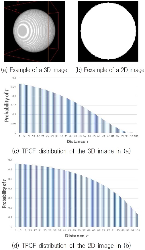
The Fig. 2(b) shows the 3D TPCF distribution according to the distance r when it is applied on Fig. 2(a). Fig. 2(d) is the 2D TPCF distribution according to the distance r when it is applied on Fig. 2(c).

Fig. 2.

Examples of TPCF distributions

3.3 Transferring the 3D TPCF characterization onto 2D space

In order to transfer the calculated S₂(r) characterization onto a 2D space, we generate a simple 2D image (Fig. 3(b)).

Fig. 3.

Example of transferring the 3D TPCF characterization of the fiber network onto the 2D image

By applying the 2D TPCF on the simple 2D image, we calculate the initial characterization P₂(r) of the simple 2D image.

Now, we update P₂(r) until P₂(r) is the most similar to the target TPCF S₂(r).

Mathematically, the updating process is defined as:

$\[ \mathrm{m}\mathrm{i}\mathrm{n}\sum _r^{}E,\mathrm{ } where E={\left[P_2\left(r\right)-S_2\left(r\right)\right]}^2 \]$

(5)

In order to minimize the energy E in Eq. (5), we repeatedly exchange the locations of two randomly selected pixels on the 2D simple image (one pixel from the background and the other from foreground). That is, with every iteration, one foreground pixel becomes a background pixel and, at the same time, one background pixel becomes a foreground pixel.

After each iteration, we have an updated 2D simple image to be used to calculate an updated energy E^ʹ. If the difference ΔE = E^ʹ - E is below a predefined threshold, we accept the exchange. Otherwise, we keep the previous simple 2D image.

By iterating this process numerous times, we create a finalized updated 2D image with the cumulative directions to lower the cumulative energy. The finalized 2D image is the 2D visualization of the original 3D fiber network.

Fig. 3 shows an example of transferring the 3D TPCF characterization of the fiber network shown in Fig. 3(a) onto the 2D image shown in Fig. 3(b). Fig. 3(c) is the distribution of S₂(r) depending on the r in the 3D image shown in Fig. 3(a). Fig. 3(d) is the distribution of P₂(r) depending on the r in the 2D image shown in Fig. 3(b).

Fig. 4 (a)-(d) show the results of the visualization of the 3D fiber network in the 2D space based on the image in Fig. 3(b) with iterations of the energy minimization process.

Fig. 4.

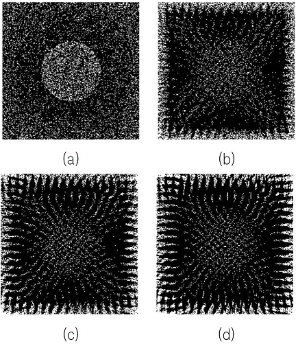
Results of the visualization of the 3D fiber network shown in Fig. 3(a) of the 2D space shown in Fig3. (b) by iterating the energy minimization process shown in Eq. (5), (a) Result of 10,000 iterations, (b) Result of 50,000 iterations, (c) Result of 100,000 iterations, (d) Result of 200,000 iterations

Fig. 4(a) is the result after 10,000 iterations of the energy minimization process in Eq. (5). Likewise, Fig. 4(b) is after 50,000 iterations, Fig. 4(c) after 100,000 iterations, and Fig. 4(d) after 200,000 iterations.

Ⅳ. Results and Discussion

We applied our proposed methods described above on the 3D images shown in Fig. 5(a)-(c).

Fig. 5.

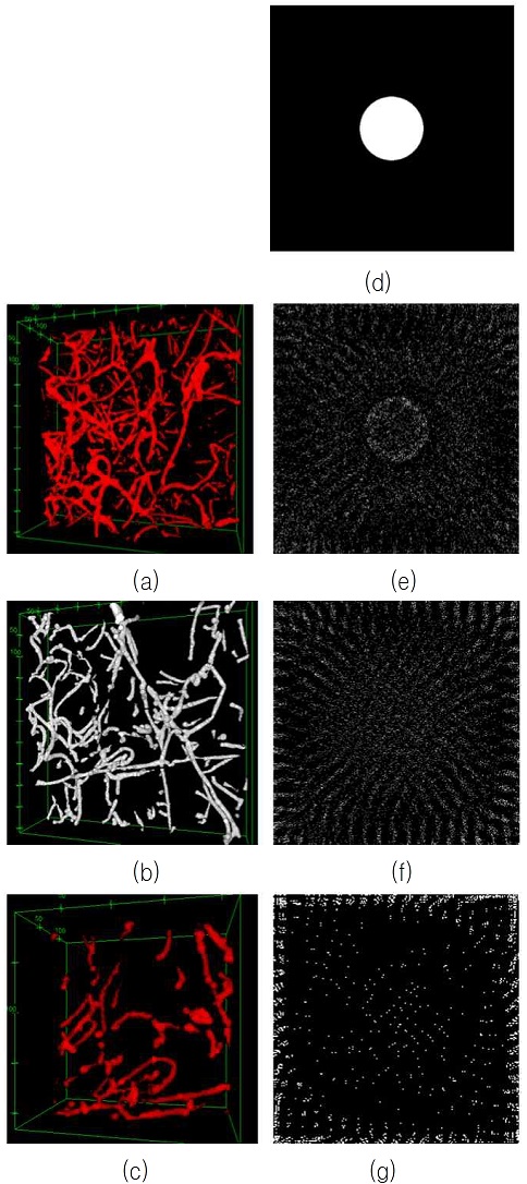
Comparison of 3-dimensional biological fiber networks on the 2-dimensional space, (a)-(c) 3D biological fiber network images, (d) initial 2D image, (e) the 2D visualization of (a) based on (d), (f) the 2D visualization of (b) based on (d), (g) the 2D visualization of (c) based on (d)

Those 3D images are produced with a confocal microscope. Their resolutions are 0.9 μm in width direction, 0.9 μm in height direction, and 0.6 μm in depth direction. In order to get the same resolution (0.9 μm) in all directions, we resampled the image in the depth direction.

Then, we applied a Gaussian kernel to the resampled images in order to avoid noises.

To compare the complexities between different biological fibers, we used the same initial simple 2D image shown in Fig. 5(d).

After 90000 iterations in order to minimize the energy defined in Eq. (5), we obtained the results shown in Fig. 5(e)-(g): Fig. 5(e) is the 2D visualization of the fiber network shown in Fig. 5(a), Fig. 5(f) is the 2D visualization of the fiber network shown in Fig. 5(b), and Fig. 5(g) is the 2D visualization of the fiber network shown in Fig. 5(c).

As we notice in Fig. 5(a)-(c), the complexity of Fig. 5(a) is the highest among those 3 fiber network examples and the complexity of Fig. 5(c) is the lowest among those 3 examples.

On the other hand, as shown in Fig. 5(e)-(g), the distribution of the white pixels in Fig. 5(e) is spread over all the areas inside the 2D image space and the structure of the inner circle is well kept, while the distribution of the white pixels in Fig. 5(g) is instead toward the boundary of the 2D image space and the structure of the inner circle is collapsed. Therefore, we find noticeable differences on the 2D image space according to the complexity of the biological fiber network in two aspects, the distribution of the white pixels and the structure of the inner circle.

We also conducted a quantitative analysis by comparing the number of the white pixels in a circle with a radius of 66 and whose center point is located in the center of a 2D image. The number of the white pixels in Fig. 5(d) is 13,673 which is almost equivalent to π • (66)².

The following Table 1 shows the number of the white pixels in a circle with a radius of 66 and whose center point is located in the center of each image in Fig. 5(e)-(g). As we see in the Table 1, as the complexity of a 3D biological fiber network becomes sparse, the number of the white pixels within a circle is noticeably reduced.

Table 1.

Number of the white pixels in a circle of with a radius of 66 whose center point is located in the middle of each image of Fig. 5(e)-(g)

Since the 3D biological fiber network contains depth information, it is normally difficult to compare those biological fiber networks directly. However, by transferring the characterization of the 3D biological fiber network onto a 2D space, we can make this comparison in a relatively easier way as seen in Fig. 5(e)-(g).

In the future, we plan to develop a parameter that gives us a numerical value to imply the complexity of a 3-dimensional biological fiber network. Thus, we expect to be able to quantify the level of complexity.

There are several research studies [12][13] on developing a special measure from TPCF directly. Our approach differs from theirs in that we are researching a way to quantify the complexity of a biological fiber network by considering the two aspects: 1) the distribution of the white pixels, and 2) the structure of an inner circle on a 2D image space.

References

• S. J. Hollister, "Porous scaffold design for tissue engineering", Nat Mater, Vol. 4, pp. 518-524, Jul. 2005. [https://doi.org/10.1038/nmat1421]
• A. Asti and L. Gioglio, "Natural and synthetic biodegradable polymers: different scaffolds for cell expansion and tissue formation", Int J Artif Organs, Vol. 37, pp. 187-205, Jan. 2014. [https://doi.org/10.5301/ijao.5000307]
• M. Boersma, D. J. A. Smit, D. I. Boomsma, Eco J.C. De Geus, H. A. Delemarre-van de Waal, and C. J. Stam, "Growing Trees in Child Brains: Graph Theoretical Analysis of Electroencephalography-Derived Minimum Spanning Tree in 5- and 7-Year-Old Children Reflects Brain Maturation", Brain connectivity, Vol 3, No. 1, pp. 50-60, Jan. 2013. [https://doi.org/10.1089/brain.2012.0106]
• M. E. J. Newman, "Networks: An Introduction", Oxford Scholarship Online, Sep. 2010.
• C. T Butts, "Social network analysis: A methodological introduction", Asian Journal of Social Psychology, Vol. 11, pp. 13-41, Feb. 2008. [https://doi.org/10.1111/j.1467-839X.2007.00241.x]
• C. T Butts and Carley KM, "Structural change and homeostasis in organizations: A decision-theoretic approach", Journal of Mathematical Sociology, Vol. 31, pp. 295-321, Oct. 2007. [https://doi.org/10.1080/00222500701542517]
• H. L. Frisch and F. H. Stillinger, "Contribution to the statistical geometric basis of radiation scattering", J. Chem, Phys, Vol. 77, pp. 2071-2077, Nov. 1962.
• S. Torquato and G. Stell, "Microstructure of two-phase random media, I. The n-point probability functions". J. Chem, Phys, Vol. 38, pp. 980-987, Aug. 1982. [https://doi.org/10.1063/1.448475]
• R. Ridgway, O. Irfanoglu, R. Machiraju, and K. Huang, "Image segmentation with tensor-based classification of n-point correlation functions", Proceedings of the Microscopic Image Analysis with Applications in Biology (MIAAB) Workshop in MICCAI, Heidelberg, Germany, Dec. 2006.
• F. Janoos, M. Okan Irfanoglu, K Mosaliganti, R. Machiraju, K. Huang, P. Wenzel, A. de Bruin, and G Leone, "Multi-resolution image segmentation using the 2-point correlation functions", In Proceedings of IEEE International Symposium on Biomedical Imaging, Arlington, VA, USA, pp. 300-303, April. 2007. [https://doi.org/10.1109/ISBI.2007.356848]
• L. A. D. Cooper, J. H. Saltz, R. Machiraju, and K. Huang, "Two-point correlation as a feature for histology images: feature space structure and correlation updating, Mathematical Methods in Bioimage", Analysis Workshop, 23rd IEEE Conference on Computer Vision and Pattern Recognition, San Francisco, CA, pp. 79-86, Jun. 2010. [https://doi.org/10.1109/CVPRW.2010.5543453]
• S. Prager, "Viscous flow through porous media", Phys. Fluid, Vol 4, pp. 1477-1482, Mar. 1961. [https://doi.org/10.1063/1.1706246]
• J. Rubinstein and S. Torquato, "Diffusion-controlled reaction: Mathematical formulation, variational principles, and rigorous bounds", J. Chem. Phys, Vol. 88, pp. 6372-6380, Jan. 1988. [https://doi.org/10.1063/1.454474]