Comparative Study on Prediction of Mortality in Heart Failure Patients using Nine Machine Learning Algorithms

Ⅰ. Introduction

Heart failure(HF) is a “chronic, progressive condition in which the heart muscle is unable to pump enough blood to meet the body’s needs for blood and oxygen”[1]. It is a disease with great global importance affecting tens of millions of people worldwide[2]. For instance, in the USA the lifetime HF risk ranges from 20% to 45% after 45 years old, according to the 2022 annual report by the American Heart Association, in conjunction with the National Institutes of Health[3]. HF-associated mortality is particularly high in developing regions such as Africa. The mortality rate is twice of the world average and 3.7 times higher than that of South America[4].

Although the methodologies for diagnosing and treating HF continue to evolve, survival times for HF patients remain several fold lower than those of age-matched groups from the general population[5]. For example, according to a study of data from the GWTG-HF(Get With The Guidelines–Heart Failure), among HF patients aged 65 to 69 years, median survival was reported to be ≤4.0 years and dropped further to ≤3.4 years for 70 to 74 year age groups. Median survival dropped even more dramatically to ≤1 year for the more than 90-year-old age group[6].

Since morbidity and mortality related to HF remain extremely important for affected patients, their families, and society as a whole, accurate prediction of these events is a crucial task. Previously, such predictions were implemented using classical biostatistical approaches.

Biostatistics involves various statistical models and tests such as the chi-square test, Pearson correlation coefficient, regression techniques(e.g., logistic, Cox), and receiver operating characteristic(ROC) curve analyses, which were frequently used to solve problems in public health. Biostatistics also includes methods for data analysis and interpretation from biological experiments and clinical trials.

In addition to biostatistical approaches, machine learning(ML) applied to healthcare datasets can be a powerful tool not only to recognize the most significant features that can lead to certain diseases but also to predict the survival rate of each patient, often more accurately, than could be achieved previously. Although logistic regression and similar simple parametric models can be sometimes more preferable to healthcare professionals compared to more complex ML methods because they are perceived to be more easily interpretable, techniques for interpreting and visualizing ML model behaviors are rapidly improving. ML methods are highly effective tools when they are combined with a clear understanding of the way to design the data pre-processing and the way to interpret the results. Therefore, we believe that ML techniques can play an important role in improving the cabability to predict HF-associated patient mortality outcomes, compared with the classical parametric regression methods which are widespread in the medical literature.

Specifically in the field of HF mortality prediction, Ahmad et al.[7] analyzed a dataset of heart patients collected in Pakistan in 2015 and published a case study of survival analysis of heart failure patients using statistical techniques. Authors concluded that age, serum creatinine, high blood pressure, anaemia and ejection fraction(EF) are important features that contribute to elevated probability of mortality among cardiovascular failure patients. The dataset analyzed by Ahmad et al.[7] has been made publicly available in the FigShare[8] repository in 2017.

Later on, Chicco and Jurman[9] experimented with the prediction using ML with only two features(i.e. serum creatinine and ejection fraction) in R. The same dataset of the newer version was donated to the UCI machine learning repository[10]. Recently Ishaq et al.[11] used the same dataset to find significant features and effective data mining techniques in Python.

The result of the study demonstrates that ETC with SMOTE achieved 92.6% accuracy.

Even though previous studies demonstrated interesting outcomes by utilizing biostatistics and machine learning techniques, there is still room for improvement using the same dataset. This study plays a role in the following areas:

To build ML models that perform better than developed models in previous studies using different techniques.

To confirm the major significant features identified from the previous studies. Is there any difference between R and Python approaches applying statistical techniques?

To confirm the feature ranking results using Random Forest. Is there any difference compared to the previous study?

The remainder of the paper describing the current study is prepared as follows: Section II explains the previous work of survival analysis of heart failure patients using the same dataset. Section III explains the dataset and feature ranking. Section IV explains outliers, pre-processing and random oversampling. Section V presents analysis of the outcome and the discussion. Finally, conclusion and future work are explained in section VI.

Ⅱ. Related work

As mentioned above, Ahmad et al.[7] utilized conventional biostatistics time-based Cox regression and Kaplan–Meier estimator to identify the significant predictors of HF patient mortality in 299 Pakistani patients, using their medical records. The authors made their dataset available on the internet together with their outcomes.

Later on Zahid et al.[12] developed gender-based survival prediction models using the same dataset. The authors found that the survival prediction model for males is notably different from that for females. For men, smoking, diabetes and anaemia are significant features while ejection fraction, sodium, and platelets count are important risk factors for females. In a sense, optimal treatments of HF for men and women could be different. However, the authors concluded that gender as being a risk factor is not really correlated with the survival of an individual patient.

These two aforementioned studies introduced interesting outcomes using biostatistics approaches. Afterwards, Davide Chicco and Giuseppe Jurman[9] used data mining techniques and ML approaches. These authors developed models to predict survival in the patients and after that to rank the most significant features contained in the medical records. However, these authors used only two features - ejection fraction and serum creatinine – in their ML analysis.

Another research conducted by Ishaq et al.[11] analyzed the same dataset to find significant features and improved machine learning models using Synthetic Minority Oversampling Technique(SMOTE) employed in nine classification models. The authors demonstrated that the ETC model achieved 92.6% accuracy in the prediction of patient survival.

Ⅲ. Dataset and featue ranking

3.1 Dataset

For this study, the heart_failure_clinical_records_dataset.csv[9] was obtained from the UCI machine learning repository[13]. The dataset provides the medical records of 299 patients who experienced HF. The record comprises 194 men and 105 women having 13 features. Patients were aged 40-95 years. Follow-up time was 4-285days with 130.2days as an average. Some features(e.g. anaemina, diabetes, high_blood_pressure, sex, smoking and death event) are categorical format and others are numerical. Table 1 gives an overview of the dataset[10].

Table 1.

Dataset description

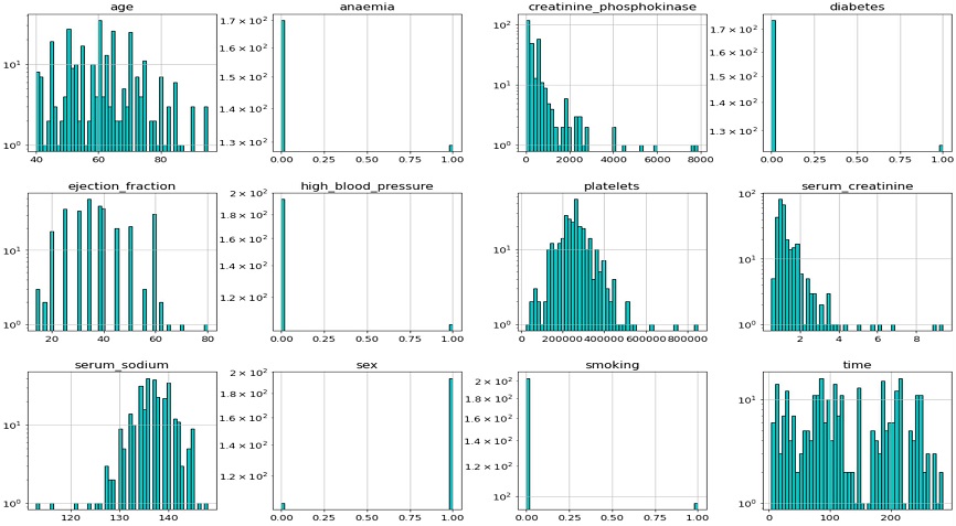
Figure 1 presents the data distribution of features. The features are clearly not normally distributed. In some medical fields, normal distributions are not expected. It is not necessary for the distribution in the collected data to be normal for the ML analyses performed here, however the sample values should be compatible with and represent the population. Samples from a population where the true distribution is normal may not look normally distributed especially when the sample size is small[14].

Fig. 1.

Visualization of the distribution of data

Table 2 explains more details about the data distribution. The Shapiro–Wilk test is a normality test in statistics[15]. The null hypothesis of the Shapiro-Wilk test is that the population data are normally distributed[15]. The test result as shown in Table 2 produced p-values. They are near 0 for all the features, which means that the null hypothesis is rejected and all features are non-normally distributed. The Shapiro–Wilk test results show that “creatinine phosphokinase” and “serum creatinine” are closer to the normal distribution, than other features.

Table 2.

Shapiro-wilk tests

The target column to be predicted by ML was the death event. The survived patients(i.e. death event = 0) numbered 203, whilst the deceased patients(i.e. death event = 1) numbered 96.

3.2 Feature ranking

3.2.1 Biostatistics

To investigate the most significant features we followed similar techniques from the previous study[3]. The authors excluded follow-up time from the dataset because they intended to concentrate on the medical features and attempted to find out the importance of those medical-related features[9]. These results could be misleading because the follow-up times for different patients varied greatly. Consequently, our study includes a follow-up time feature(Time) to find out whether there is any relation to the chance of survival of a patient.

Traditional univariate biostatistics such as Pearson correlation coefficients(PCC), Shapiro-Wilk, Chi-square test and Mann-Whitney U test were applied to examine which features have the strongest associations.

The PCC in statistics, is a number that quantifies the linear association between two variables X and Y. It has a value between +1 and -1, +1 means perfect positive linear correlation which Y increases as X increases and 0 means no linear correlation and -1 means perfect negative linear correlation in which Y increases as X decreases[17]. Table 3 shows the result of feature ranking based on the value of the PCC.

Table 3.

Pearson correlation coefficients(PCC)

To see the stronger tendency, the absolute value function has been used to capture both positive and negative correlations in the same ranking scale. Table 4 gives the result of feature ranking based on the absolute value of PCC. The feature ranking is the same as the previous study except for the feature “Time” as this is included in this study.

Table 4.

Pearson correlation coefficients abs(PCC)

The Chi-square test(Chi test or χ2 test) evaluates if the relationship between two variables is statistically significant. The null hypothesis of the Chi test is that there is no relationship between two variables meaning they are independent. If the p-value is less than or equal to a significant level(e.g. 0.05) then the null hypothesis is rejected meaning two variables have a significant relationship[18].

In another word, a low p-value implies that the two variables have a strong relationship and a high p-value cannot determine that the two variables are related. The result is the same except bottom 3 ranking(Table 5). The previous study shows the sequence as “Smoking”, “Sex” and Diabetes” after “Plates”. This is because the previous study used R language and this study has used Python. Some models in R are already standardized whereas Python does not.

Table 5.

Chi squared test

The Mann-Whitney U test(or Mann-Whitney-Wilcoxon)[19] evaluates if the medians of the two populations are different. The null hypothesis of a Mann–Whitney U test is that the two samples have the same median meaning that the distributions of the two populations are equal. The test has been applied to each feature with regard to the death events. A low p-value implies that the examined feature is strongly related to death event. The results of feature ranking(Table 6) are different from the previous study(Table 7)[9].

Table 6.

Mann–whitney U test

Table 7.

Mann–whitney U test

The reason for the difference in results can be some models in R language standardizes the data as default whereas Standard-Scaler or Min-Max scaler shall be applied in Python.

3.2.2 Machine Learning

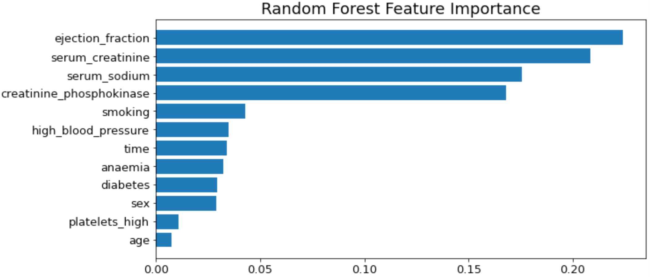
Similar to the previous study[11][16] Random Forest has been used to obtain feature ranking results (Figure 3). According to[11], the significant features are time, creatinine, ejection fraction and age. However, this study discovered ejection fraction, serum creatinine, creatinine phosphokinase and serum sodium as significant features.

Fig. 2.

Significant features by random forest

Fig. 3.

Age feature engineering

IV. Experimental Design

The objective of this study is to build an improved survival prediction model using different ML techniques which have not been employed in previous studies[7][9][11][12].

Survival analysis in statistics analyzes the time before an event(e.g. death, recovery) occurs[20]. For the example death event, survival analysis employs the time from the beginning of observation to death for each patient. The Cox Proportional-Hazard Model(or Cox model) is a simple type of survival analysis, which estimates how the features(predictor variables) are associated with the hazard function for the outcome variable(death event in this case). Risk factors affecting the survival rate can be identified through the Cox regression analysis[21].

In the previous study[7] the authors highlighted age as the most significant risk factor in the Cox model however, the authors used the biostatistics method to develop the model instead of using the machine learning model. This study builds and evaluates the performance of models using the age-specific risk factor of patients.

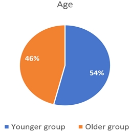
Age feature has 40-95 range. The feature has been categorized into two groups. The younger group describes patients in the 35-60 range while the older group describe patients in 60-100(Figure 3).

One of the important steps in data preprocessing is detecting and handling outliers because the outliers may negatively affect the training process of machine learning algorithms and lead to lower accuracy. We have detected “platelets”, “creatinine phosphokinase” and “serum creatinine” have more outliers than other features. Outliers were detected and replaced with mean values as their data types are numeric.

As the target feature is imbalanced(i.e. 203 patients as survived vs 96 as deceased), the random oversampling technique has been applied to balance the minority class. Random oversampling chooses some of the samples from the minority class randomly to replace them with multiple copies of the minority classes in training data[22]. Otherwise, the imbalance might affect the performance of ML algorithms.

V. Analysis of Outcome

In this section, the model design and outcomes of all model experiments for the prediction of HF patients’ survival are reviewed. The dataset has been presented in Table 1. Random oversampling has been applied to make the target feature balanced. The dataset has been split randomly into 70% for the training set and 30% for the testing set. Various Machine learning models have been applied to the training set. Accuracy, precision, recall and F-score are calculated to compare the performance. The development and evaluation have been carried out in Google Colaboratory and encoded by Python. The source code is publicly accessible on GitHub(https://github.com/alwaysapril/prediction-models-for-heart-failure-patients)

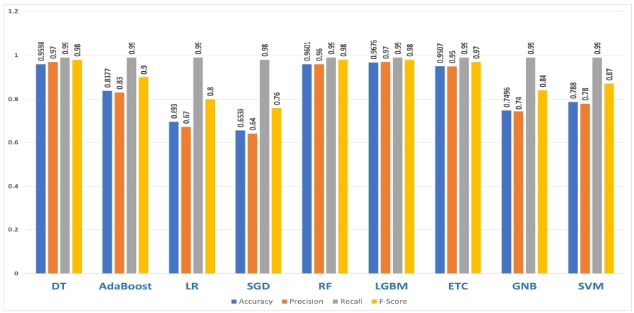
Nine classification models such as DT, AdaBoost, LR, SGD, RF, LGBM, ETC, GNB and SVM have been employed. These algorithms are appropriate for the dataset this study analyzes and they have been proven successful in the prediction of survival rates in the past[11]. In this study, the Light Gradient Boosting Machine(LGBM) has been used instead of the GBM algorithm because it is a free and open source. Figure 4 provides the overall performance analysis of age- based machine learning models with random oversampling.

Fig. 4.

Performance of nine classification model

Results showed performance of tree-based algorithms(RF, LGBM and ETC) performed better than regression-based(LR and SGD) or statistical-based(GND and SVM).

Table 8 shows that LGBM outperformed other models with 0.9676 accuracy which has been improved compared with ETC algorithms which had a 0.9262 accuracy in[11]. All figures in accuracy, recall and F-score have been improved compared to the previous study.

Table 8.

Age based survival prediction models with random oversampling

In this study, ML models using the age-specific risk factor have been suggested to predict the survival of heart failure patients aiming to determine the effects of age on prediction of mortality in HF patients. Additionally, random forest selected the most significant features as ejection fraction, serum creatinine, creatinine phosphokinase and serum sodium as significant features.

This study took advantage of past studies. Nine classification machine learning models include DT, AdaBoost, LR, SGD, RF, LGBM, ETC, GNB and SVM. Accuracy results show improvement in all nine models. LGBM with random oversampling showed the highest result in four evaluation measures and achieved 0.9676 accuracy, 0.97 precision, 0.99 recall and 0.98 F-Score. Our results show that ML can predict the survival of heart failure patients with high accuracy. Our findings will be useful for physicians and the research approach can be replicated for other health related datasets to solve similar health machine learning problems.

References

• V. Rudomanova and B. C. Blaxall, "Targeting GPCR-Gβγ-GRK2 signaling as a novel strategy for treating cardiorenal pathologies", Biochim. Biophys. Acta (BBA)-Molecular Basis Dis., Vol. 1863, No. 8, pp. 1883-1892, Aug. 2017. [https://doi.org/10.1016/j.bbadis.2017.01.020]
• B. Ziaeian and G. C. Fonarow, "Epidemiology and aetiology of heart failure", Nat. Rev. Cardiol., Vol. 13, No. 6, pp. 368-378, Mar. 2016. [https://doi.org/10.1038/nrcardio.2016.25]
• C. W. Tsao et al., "Heart disease and stroke statistics—2022 update: a report from the American Heart Association", Circulation, Vol. 145, No. 8, pp. e153-e639, Jan. 2022. [https://doi.org/10.1161/CIR.0000000000001052]
• A. A. Ajayi, G. G. Sofowora, and G. O. Ladipo, "Explaining heart failure hyper-mortality in sub saharan Africa: global genomic and environmental contribution review", J. Natl. Med. Assoc., Vol. 112, No. 2, pp. 141-157, Apr. 2020. [https://doi.org/10.1016/j.jnma.2020.02.003]
• C. W. Yancy et al., "2017 ACC/AHA/HFSA focused update of the 2013 ACCF/AHA guideline for the management of heart failure: a report of the American College of Cardiology/American Heart Association Task Force on Clinical Practice Guidelines and the Heart Failure Society of America", J. Am. Coll. Cardiol., Vol. 136, No. 6, pp. e137-e161, Aug. 2017. [https://doi.org/10.1161/cir.0000000000000509]
• K. S. Shah et al., "Heart failure with preserved, borderline, and reduced ejection fraction: 5-year outcomes", J. Am. Coll. Cardiol., Vol. 70, No. 20, pp. 2476-2486, Nov. 2017. [https://doi.org/10.1016/j.jacc.2017.08.074]
• T. Ahmad, A. Munir, S. H. Bhatti, M. Aftab, and M. A. Raza, "Survival analysis of heart failure patients: A case study", PLoS One, Vol. 12, No. 7, pp. e0181001, Jul. 2017. [https://doi.org/10.1371/journal.pone.0181001]
• Figshare, "Figshare" https://figshare.com, , [accessed: Jul. 25. 2022]
• D. Chicco and G. Jurman, "Machine learning can predict survival of patients with heart failure from serum creatinine and ejection fraction alone", BMC Med. Inform. Decis. Mak., Vol. 20, No. 1, pp. 1-16, Feb. 2020. [https://doi.org/10.1186/s12911-020-1023-5]
• D. Chicco, "Heart failure clinical records Data Se." https://archive.ics.uci.edu/ml/datasets/Heart+failure+clinical+records, [accessed: Jun. 22, 2022]
• A. Ishaq et al., "Improving the prediction of heart failure patients’ survival using SMOTE and effective data mining techniques", IEEE access, Vol. 9, pp. 39707-39716, Mar. 2021. [https://doi.org/10.1109/access.2021.3064084]
• F. M. Zahid, S. Ramzan, S. Faisal, and I. Hussain, "Gender based survival prediction models for heart failure patients: A case study in Pakistan", PLoS One, Vol. 14, No. 2, pp. e0210602, Feb. 2019. [https://doi.org/10.1371/journal.pone.0210602]
• A. Asuncion and D. Newman, "UCI machine learning repository", Irvine, CA, USA, 2007.
• D. G. Altman and J. M. Bland, "Statistics notes: the normal distribution", Bmj, Vol. 310, No. 6975, pp. 298, Feb. 1995. [https://doi.org/10.1136/bmj.310.6975.298]
• S. S. Shapiro and M. B. Wilk, "An analysis of variance test for normality(complete samples)", Biometrika, Vol. 52, No. 3/4, pp. 591-611, Dec. 1965. [https://doi.org/10.2307/2333709]
• D. Chicco and C. Rovelli, "Computational prediction of diagnosis and feature selection on mesothelioma patient health records", PLoS One, Vol. 14, No. 1, pp. e0208737, Jan. 2019. [https://doi.org/10.1371/journal.pone.0208737]
• K. Pearson, "Notes on Regression and Inheritance in the Case of Two Parents", Proc. of the Royal Society of London, Vol. 58, pp. 347-352, Jan. 1895. [https://doi.org/10.1098/rspl.1895.0041]
• Minitab, "Interpret the key results for Chi-Square Test for Association", https://support.minitab.com/en-us/minitab/19/help-and-how-to/statistics/tables/how-to/chi-square-test-for-association/interpret-the-results/key-results, [accessed: Jun. 29, 2022].
• H. B. Mann and D. R. Whitney, "On a test of whether one of two random variables is stochastically larger than the other", Journal article, Vol. 18, No. 1, pp. 50-60, Mar. 1947. [https://doi.org/10.1214/aoms/1177730491]
• A. Grayson, D. D. Clarke, and H. Miller, "Help-seeking among students: are lecturers seen as a potential source of help?", Stud. High. Educ., Vol. 23, No. 2, pp. 143-155, 1998. [https://doi.org/10.1080/03075079812331380354]
• D. R. Cox, "Regression models and life‐tables", J. R. Stat. Soc. Ser. B, Vol. 34, No. 2, pp. 187-202, Jan. 1972. [https://doi.org/10.1007/978-1-4612-4380-9_37]
• C. X. Ling and C. Li, "Data mining for direct marketing: Problems and solutions", in Kdd, Vol. 98, pp. 73-79, 1998.