A Study on Weeds Retrieval based on Deep Neural Network Classification Model
Abstract
In this paper, we study the ability of content-based image retrieval by extracting descriptors from a deep neural network (DNN) trained for classification purposes. We fine-tuned the VGG model for the weeds classification task. Then, the feature vector, also a descriptor of the image, is obtained from a global average pooling (GAP) and two fully connected (FC) layers of the VGG model. We apply the principal component analysis (PCA) and develop an autoencoder network to reduce the dimension of descriptors to 32, 64, 128, and 256 dimensions. We experiment weeds species retrieval problem on the Chonnam National University (CNU) weeds dataset. The experiment shows that collecting features from DNN trained for weeds classification task can perform well on image retrieval. Without applying dimensionality reduction techniques, we get 0.97693 on the mean average precision (mAP) value. Using autoencoder to reduced dimensional descriptors, we achieve 0.97719 mAP with the descriptor dimension is 256.
초록
본 논문에서는 분류 목적으로 훈련 된 심층신경망에서 서술자을 추출하여 컨텐츠 기반 이미지 검색의 수행 능력을 연구하였다. 잡초 분류를 위해 학습된 VGG 심층신경망 모델을 미세 조정하여 사용한다. 해당 VGG 모델의 2개의 전결합층과 전역 평균 풀링으로 부터 이미지의 서술자인 특징벡터를 얻는다. 특징벡터의 차원을 줄이기 위하여 주성분 분석을 적용하고, 오토인코더 네트워크를 개발하여 차원을 32, 64, 128, 256차원으로 줄였다. 실험은 전남대학교 잡초 데이터 세트에서 ‘종’ 검색을 진행 하였다. 실험에 따르면 잡초 분류를 위해 훈련된 심층신경망에서 수집된 특징은 이미지 검색에서 우수한 성능을 보인다. 차원 축소 기법 없이 평균정밀도의 평균값은 0.97693을 달성한다. 반면 오토인코더를 통한 설명자 차원을 줄이면, 설명자 256차원에서 평균 정밀도의 평균값은 0.97719를 달성한다.
Keywords:
weeds retrieval, deep neural network, dimensionality reduction, autoencoder, PCA, feature extractionⅠ. Introduction
In real life, many kinds of weeds are unknown or cannot be recognized by farmers. One of the approaches to solve this problem is applying content-based image retrieval to return images from the gallery that are similar to a given query image. In content-based image retrieval, visual contents, such as edges or colors, are used as descriptors of the image. A metric function is implemented to retrieve base on those descriptors. There are many approaches to define descriptors such as SIFT/SURF [1], BoW [2], HOG [3], or extract descriptors from a neural network such as autoencoder [4] and convolutional neural network (CNN) [5].
Recently, Babenko et al. [6] pointed out that the descriptor returned from DNN used for classification tasks could perform well in retrieval application. Inspired by this research, we investigate the content-based weeds image retrieval problem using trained DNN for weeds classification tasks. With this approach, we define a similarity based on species that images belong to. The descriptor of the image comes from layers in this DNN, and Euclidean distance is used to measure the similarity between a query image to images in the gallery set based on these descriptors. In the experiment, this retrieval approach shows high performance on retrieval tasks; mAP is 0.97693. Also, we evaluate retrieval performance when compressing descriptors to lower dimensions (e.g., 32, 64, 128, or 256 dimensions) using PCA or autoencoder. We notice that some descriptors slightly reduce on mAP. Autoencoder performs better than PCA and even gets higher on mAP value than original descriptors, such as 0.97719 mAP with compressed GAP descriptor. Overall, the contributions of this study are analyzing behaviors of the weeds retrieval problem by collecting descriptors from a DNN model trained for weeds classification tasks and developing an autoencoder that efficient to weeds descriptor dimensional reduction.
The organization of this paper is as follows: First, we briefly describe the information on related DNN and image retrieval problems in Section II. Then, in Section III, we explain how to extract features from a DNN model, apply dimensionality reduction methods such as PCA and autoencoder to reduce the dimension of feature vectors, and use similarity metrics for retrieval. Section IV describes our experimental results, including the introduction of the CNU weeds dataset, retrieval performances, and examples of retrieved images. Finally, Section V is our conclusion after experiments.
Ⅱ. Related works
2.1 DNN
Simonyan and Zisserman [7] proposed a depth DNN architecture using stack of small size 3×3 convolutional filters, which now we called as VGG net. They showed that using stacks of small size of receptive fields 3×3 had similar effects to a larger 5×5 or 7×7 receptive field. By their model configuration, earlier layers studies low-level features such as micro features, small textures on the object. In comparison, later layers studies high-level features such as edges, shapes, overall characteristics of the object. The last layer of stacking convolutional layers has 512 channels, the authors then added FC layers and softmax layer for training in the ILSVRC dataset. VGG net achieved the state-of-the-art on the ILSVRC competition in 2014.
2.2 Image retrieval
Recently, many scientific papers have shown the correlation between image classification and image retrieval. Xie et al. [8] proposed Online nearest neighbor estimation algorithm that could be used for classification and retrieval tasks. Tolias et al. [9] used a convolutional layer in a DNN model to encoded many regions on the image into short vectors used for retrieval as well as localization. Babeko and Lempitsky [10] investigated how to combine multiple local feature descriptors to create global descriptors efficiently in the image retrieval problem.
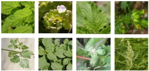
Our work was inspired by Babenko et al. [6], where the authors showed positive image retrieval results when using trained CNN on the classification task. They extracted feature vectors from the last max pooling and 2 FC layers as image descriptors. The retrieval results using this approach were slightly lower or even higher than previous descriptors approach, depending on datasets. They found that earlier descriptors were suitable for low-level retrieved texture, while later descriptor was sensitive to high-level textures. In their experiment, the original descriptors had a length of 4096, which made it time-consuming to retrieve. They solved this problem by applying dimensionality reduction techniques such as PCA and discriminative reduction (SIFT + nearest neighbor matching with the second-best neighbor test + RANSAC validation). The result showed a similar retrieval result after reducing to 256 dimensions. However, this discriminative reduction was not suitable in the weeds image because local features on the surface consist of many low-level features (shown in Fig. 5), which can make SIFT fail to capture useful descriptors. Instead, we use a nonlinear reduction technique such as autoencoder since this network can obtain diverse information available from descriptors.
Ⅲ. Methodology
3.1 DNN and image retrieval
Fig. 1 shows overall DNN architecture. For the classification task, training images are feed to DNN, where the last layer is GAP. Then, we add an FC layer with a length of 256 (denoted as FC256), followed by a batch normalization (BN) layer, and activation function is the rectified linear unit (RELU). Finally, we fed the output of RELU to an FC layer with length equal to the number of classes in the dataset (denoted as FCclass), followed by a softmax layer to determine the probability that input image belongs to species. After training the classifier, GAP, FC256, and FCclass are used as the descriptor of the input image for retrieval task.
Fig. 2 shows the overall scheme for our study on weeds retrieval based on the DNN classification model. Assume that we select “descriptor 2” as the descriptor of images, given a query image and a gallery set, we collect descriptors by feeding those images to the DNN model. Then, we measure distances between the query image and all images in the gallery set, using these descriptors. Finally, k images in the gallery corresponding to k smallest distances, are returned as retrieval results of the query image.

Overall scheme for retrieval task. First, a query image and images in the gallery set are passed through the DNN model. Then, DNN model returns descriptors. Next, we can apply dimensionality reduction on descriptors (optional). Later, L2 normalization is use as a preprocessing step. We use Euclidean distance to measure the distance between the query descriptor and descriptors in the gallery set. Finally, we return k images in the gallery set corresponding to k smallest distances
3.2 Retrieval similarity metric
Given two descriptor vectors x = (x1,x2,…xn) and y = (y1,y2,…yn) have n dimensions in the Cartesian coordinate, the similarity between these two vectors is measured by Euclidean distance, d(x,y), in equation (1). The lower of d, the higher similarity of x and y.
| (1) |
L2 normalization is used as a preprocessing step before measuring similarity to deal with the high dispersity of descriptors set. This normalization is also used in cosine similarity metric to scale the length of a vector. After normalization, Euclidean norm of all descriptors is 1, where Euclidean norm is defined in (3).
| (2) |
| (3) |
3.3 Dimensionality reduction
PCA is a linear approach to reduce the dimension of descriptor vectors. Assume that the dataset has N vectors, and the original vector xi in this dataset has a size of n × 1. We can project to lower dimension k < n by choosing a subspace that minimizes the reconstruction error, which can be done by using the n × n covariance matrix C in (4).
| (4) |
where μ is the average vector of vectors in the dataset. The optimal subspace is determined by the top k largest eigentvalues, corresponding to k eigenvectors of C. Thus, we can choose these eigenvectors to form a projection matrix . A projection of vector xi from n to d dimension is made by
| (5) |
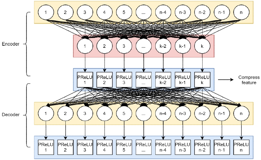
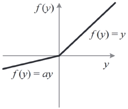
Autoencoder is a nonlinear approach for dimensionality reduction. Mathematically, it learns a function hw,b(x)≈x, where x is the input, and W,b is a set of parameters. An autoencoder contains two modules: Encoder and decoder. Encoder learns a mapping to lower dimension with k < n. The decoder learns how to map back to x from the latent z. Both encoder and decoder can be parameterized by a neural network with a set of parameters. Each layer in the network has an activation function so that autoencoder can become a nonlinear mapping to reduce dimension. In this paper, we choose the parametric rectified linear unit (PReLU) [11] as the activation function. This activation function gives each node a specific trainable parameter to maintain essential values for the next layer shown in Fig. 4.
Fig. 3 shows an overall architecture of the autoencoder used for reducing the dimension of an input feature vector. This autoencoder contains two sub-neural networks: Encoder receive n-dimension input vector, then operate with n × k learnable weights Wencoder and k biases bencoder for mapping input to k dimensions.
A PReLU (as shown in Fig. 4) with k learnable parameters are used as the activation function for nonlinearly mapping. z is the output of PReLU (also the output of the encoder module). In total, the encoder module has n × k + k+ k = k(n + 2) learnable parameters Wencoder and bencoder, then pass to the activation function PReLU. The output of PReLU is h(x) has the same dimension with x.
Autoencoder uses regression optimization techniques such as mean square error (MSE) to calculate loss between h(x) and x, and backpropagation methods like adadelta [12] to find W and b that optimize the loss function, where W = {Wencoder, Wdecoder} + {bencoder, bdecoder} so that h(x) ≈ x.
Ⅳ. Experimental results
4.1 Dataset
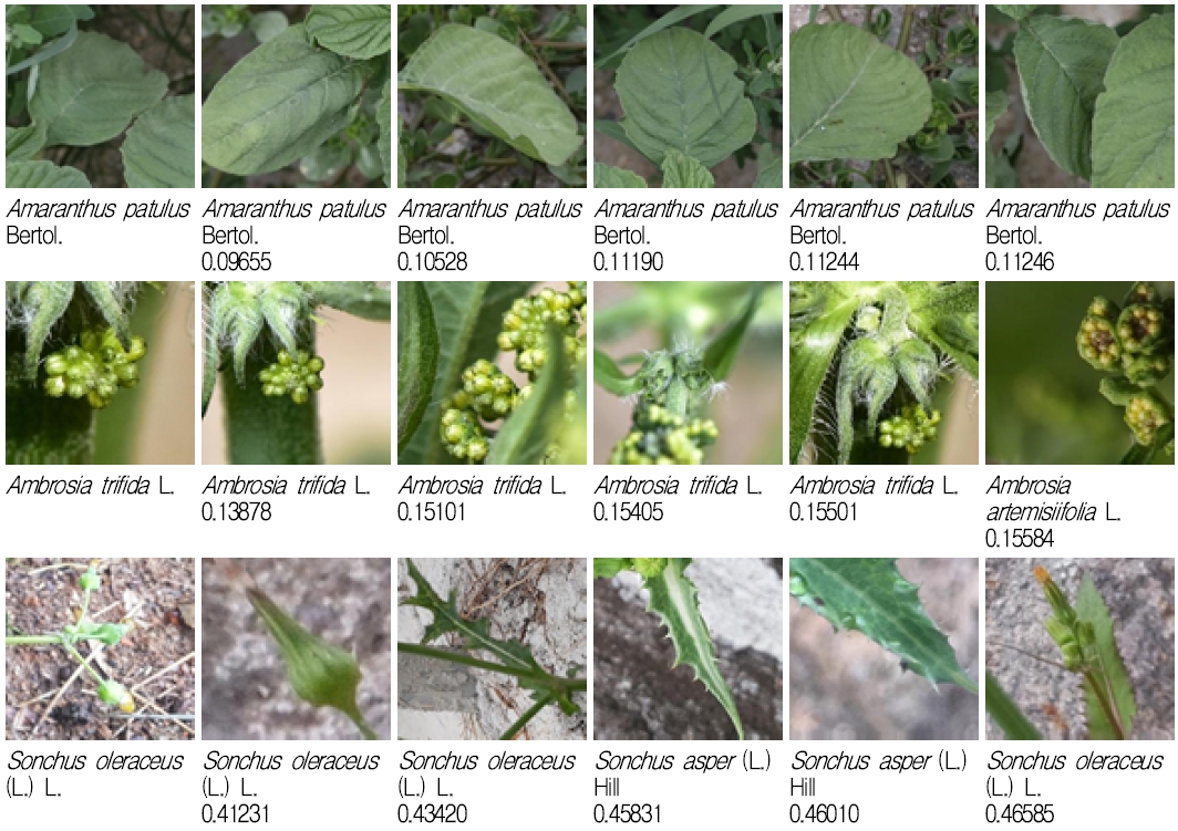
We used Chonnam National University (CNU) weeds dataset for retrieval experiments. This dataset has 21 species belong to five families, 208477 images in total [13]. As shown in Table 1, this dataset is imbalance, where the species has the largest number of images is Galinsoga quadriradiata Ruiz & Pav., around 24300 images, while species Bidens bipinnata L. has the smallest number of images, about 800 images. Fig. 5 shows images example in this dataset.
Given an image I, we retrieve k images in the training set that most “similar” with I through a metric distance function. The “similar” term refers to images that belong to a particular species.
For classification and retrieval experiment, 60% images in each species were used as the training set (also the gallery set for retrieval), 20% were the validation set to selected the optimal DNN parameters in classification task, and the remains 20% were the test set (also the query set for retrieval).
4.2 Weeds classification
We applied transfer learning on the VGG net for training weeds classification [14], in which parameters in this network were retrained on the ImageNet dataset, which already contains weeds images [15]. As shown in Fig. 1, we added the GAP layer, followed by an FC256, batch normalization layer, ReLU as the activation function, then passed to another FC layer before using softmax to get a probability vector. This FC layer had a size of 21 (equal to the number of species, we called it FC21), and the output of a softmax layer was used to calculate loss via the categorical cross-entropy loss function. The input was a 128×128 RGB color image, rescaled to [0,1] range. When applying transfer learning, we froze the first five layers and trained with a batch size of 128, and no data augmentation techniques were used. The learning rate was 0.001, and the optimization algorithm was stochastic gradient descent on 50 epochs.
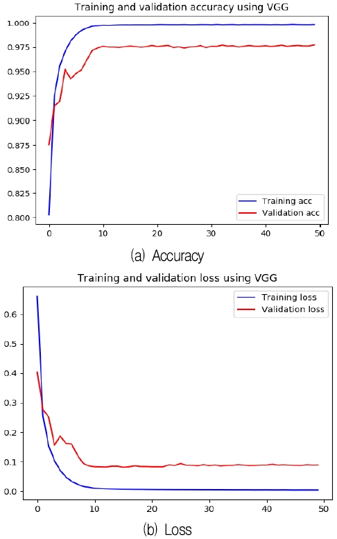
Fig. 6 shows training and validation loss and accuracy on 50 epochs. VGG started to converge from 10th epoch, and validation accuracy varied around 0.975.
After 50 epochs, Table 2 shows the accuracy, precision, recall, and F1 score on the test set, where the accuracy was 0.97643, and the F1 score was 0.96437.
4.3 Weeds retrieval
To demonstrate the efficiency of retrieval by using features from the DNN learned by classification task, given an image I, we validated feature from GAP, FC256, and FC21 from VGG as the feature descriptor of I. Since the dispersity of descriptors may be extensive, we applied L2 normalization to scale descriptor x before retrieval. L2 normalization aims to make a k-dimension point lay on a unit ball centered at the origin, calculated by expression (2), where ∥x∥2 is Euclidean norm. Euclidean distance was used to measure the similarity between x and each descriptor on the gallery set. k images with the shortest distance concluded as retrieval results of the image in the query set. Assume the number of images in the query set is Q, Iq and Ig is the image belongs to query and gallery set, we used mAP as the retrieve evaluation in terms of t, where t is the name of species or family of image. The mAP is calculated by expression (6):
| (6) |
where
| (7) |
Table 3 shows mAP results when we retrieved five images in the gallery set. The highest performance was GAP, followed by FC256 and FC21. Because of the natural characteristic of weeds, low-level feature plays a vital role in presenting weeds feature, which made GAP had the highest performance among all. The mAP performance shows that using DNN for classification task can also perform well on retrieval.
Fig 7. show examples of retrieval results. Retrieved images were entirely identical to the outside characteristic of the weeds species, show that a DNN model on classification task can capture essential features, which can be used as a descriptor for retrieval.
4.4 Dimensionality reduction
In this step, we experimented on dimensionality reduction on descriptors for faster retrieval. We did not apply this technique on FC21 because this descriptor has low dimensions. Instead, we used PCA and autoencoder to reduce the dimension of GAP and FC256 descriptors to 32, 64, and 128 (and 256 for GAP).
Table 4 and Table 5 show the mAP of GAP and FC256 after using PCA for dimensionality reduction. When reducing GAP dimension to 128, 256, and FC256 to 64, 128, the results were even higher than using original descriptors, except 32 dimensions were much lower. Fig. 8 shows examples of retrieved images after applying dimensionality reduction to reduce the descriptor dimension to 128.
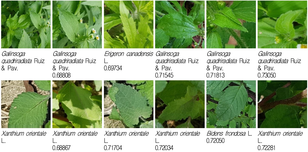
Retrieval examples when applying PCA to reduce GAP and FC128 descriptors to 128 dimensions. 1st row shows GAP case, 2nd row shows FC256 case. Images on the left-most column from the query set and the next five images from left to right are retrieval results in descending order of Euclidean distance.
In this experiment, we used the autoencoder demonstrated in Fig. 3. Given the input descriptor, we treated the output of the first PReLU (in encoder module) as a reduction result of the input descriptor, which was GAP and FC256. Similar to PCA approach, this PReLU had a length of 32, 64, 128 (and 256 for GAP). On training, we applied cyclical learning rates (CLR) triangular policy proposed on [16]. We trained on 1000 epochs per each dimension, with adadelta as the optimization method for MSE loss function. After 1000 epochs, we chose parameters on encoder and decoder modules having minimum on loss function on the validation set. By experiment, the optimal setting of batch size, max, and min learning rates boundary for CLR correspond to specific reduction are shown in Table 6 (for GAP descriptor) and Table 7 (for FC256 descriptor).

Setting of batch size, min and max learning rate, and loss of validation set on each dimension, applied on GAP

Setting of batch size, min and max learning rate, and loss of validation set on each dimension, applied on FC256
After reducing the dimension, retrieval results in Table 8 and Table 9 show mAP performance when retrieved five images from the gallery set. Applying autoencoder to reduce feature dimension attained performance higher than the original, except for the 32 dimensions that suffered a lack of information.
On GAP and FC256 descriptor, 64 and 256 dimensions that using autoencoder had better performance than PCA, and only 32 dimensions shows the dominance of PCA than autoencoder. While reducing descriptor to 32, 64, and 128 dimensions; in most cases, using GAP as descriptor yields better performance than FC256 since GAP is an earlier layer which can capture low-level features that play an essential role in weeds classification as well as weeds retrieval.
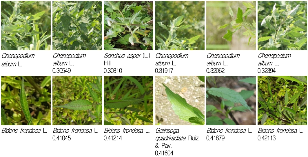
Retrieval examples in terms of species when applying autoencoder to reduce GAP and FC128 descriptors to 128 dimensions. 1st and 2nd row used GAP, 3rd and 4th row used FC256. L2 normalization applied to descriptor on odd rows. Images on the left-most column from the query set and the next five images from left to right are retrieval results in descending order of Euclidean distance
Ⅴ. Conclusion
In this paper, we investigated the ability to use descriptors in a DNN model trained for weeds classification problems and to transfer these descriptors to weeds retrieval problems. Results showed that in a classification problem, the DNN model could capture suitable features on the weeds, which can be used as the descriptor for retrieval problems and achieve significantly high in mAP value. We experimented on the CNU weeds dataset using GAP, FC256, and FC21 layers extracted from the trained VGG model as feature descriptors of the weeds image. The similarity characteristics of weeds image are that earlier layers are capable of capturing low-level features, and the mAP values show that using GAP as the descriptor is highly useful in weeds retrieval. Applying autoencoder to reduce the dimension of GAP and FC21 descriptors to 64, 128 (and 256 in case of GAP) enhanced the performance. This study contributes a promising approach to real-world weeds retrieval applications. In the future, we will employ this experiments on mobile devices and use in smart agriculture applications.
Acknowledgments
This work was carried out with the support of “Cooperative Research Program for Agriculture Science and Technology Development (Project No. PJ01385501)” Rural Development Administration, Republic of Korea.
References
-
N. Ali, K. B. Bajwa, R. Sablatnig, S. A. Chatzichristofis, Z. Iqbal, M. Rashid, and H. A. Habib, "A novel image retrieval based on visual words integration of SIFT and SURF", PloS one, Vol. 11, No. 6, e0157428, 2016.
[https://doi.org/10.1371/journal.pone.0157428]

-
Y. Ren, A. Bugeau, and J. Benois-Pineau, "Bag-of-bags of words irregular graph pyramids vs spatial pyramid matching for image retrieval", in 2014 4th international conference on image processing theory, tools and applications (IPTA), Paris, France, pp. 1-6, Oct. 2014
[https://doi.org/10.1109/IPTA.2014.7001967]

-
R. Hu and J. Collomosse, "A performance evaluation of gradient field hog descriptor for sketch based image retrieval", Computer Vision and Image Understanding, Vol. 117, No. 7, pp. 790-806, Jul. 2013.
[https://doi.org/10.1016/j.cviu.2013.02.005]

- G. Xu and W. Fang, "Shape retrieval using deep autoencoder learning representation", in 2016 13th International Computer Conference on Wavelet Active Media Technology and Information Processing (ICCWAMTIP), Chengdu, China, pp. 227-230, Dec. 2016.
-
M. Tzelepi and A. Tefas, "Deep convolutional learning for content based image retrieval", Neurocomputing, Vol. 275, pp. 2467-2478, Jan. 2018.
[https://doi.org/10.1016/j.neucom.2017.11.022]

-
A. Babenko, A. Slesarev, A. Chigorin, and V. Lempitsky, "Neural codes for image retrieval", in European conference on computer vision, Zurich, Switzerland, pp. 584-596, Sep. 2014.
[https://doi.org/10.1007/978-3-319-10590-1_38]

- K. Simonyan and A. Zisserman, "Very deep convolutional networks for large-scale image recognition", in arXiv preprint arXiv:1409.1556, , 2014.
-
L. Xie, R. Hong, B. Zhang, and Q. Tian, "Image classification and retrieval are one", in Proceedings of the 5th ACM on International Conference on Multimedia Retrieval, Shanghai China, pp. 3-10, Jun. 2015.
[https://doi.org/10.1145/2671188.2749289]

- G. Tolias, R. Sicre, and H. Jégou, "Particular object retrieval with integral max-pooling of CNN activations", in arXiv preprint arXiv:1511.05879, , Nov. 2015.
- Artem Babenko and Victor Lempitsky, "Aggregating deep convolutional features for image retrieval", 2015 IEEE International Conference on Computer Vision (ICCV), Santiago, Chile, pp. 1269-1277, Dec. 2015.
- K. He, X. Zhang, S. Ren, and J. Sun, "Delving deep into rectifiers: Surpassing human-level performance on imagenet classification", in Proceedings of the IEEE international conference on computer vision, Santiago, Chile, pp. 1026-1034, Dec. 2015.
- M. D. Zeiler, "Adadelta: an adaptive learning rate method", in arXiv preprint arXiv:1212.5701, , Dec. 2012.
-
H. T. Vo, G. H. Yu, H. T. Nguyen, J. H. Lee, T. V. Dang, and J. Y. Kim, "Analyze weeds classification with visual explanation based on Convolutional Neural Networks", Smart Media Journal, Vol. 8, No. 3, pp. 31-40, Sep. 2019.
[https://doi.org/10.30693/SMJ.2019.8.3.31]

- K. Simonyan and A. Zisserman, "Very deep convolutional networks for large-scale image recognition", arXiv preprint arXiv:1409.1556, , Apr. 2015.
- ImageNet, [Online]. Available: http://www.image-net.org/search?q=weed, . [accessed 30 Sep. 2019].
-
L. N. Smith, "Cyclical learning rates for training neural networks", in 2017 IEEE Winter Conference on Applications of Computer Vision (WACV), Santa Rosa, CA, USA, pp. 464-472, Mar. 2017.
[https://doi.org/10.1109/WACV.2017.58]


2017 : BS degree in Department of Mathematics, Computer Science, Ho Chi Minh University of Science, Vietnam
2020 : MS degree in Department of Electronic Engineering, Chonnam National University
2020. 03 ~ now : Ph.D student in Department of Electrical Engineering, Chonnam National University
Research interests: Digital signal processing, image processing, machine learning

2018 : MS degree in Department of Electrical Engineering, Chonnam National University
2018. 03 ~ now : PhD student in Department of Electronic Engineering, Chonnam National University
2018. 12 ~ now : Insectpedia C.E.O
Research interests : Digital signal processing, video processing, audio signal processing, machine learning, deep learning
2017 : BS degree in Department of Mathematics, Computer Science, Ho Chi Minh University of Science Department, Vietnam
2019. 03 ~ now : MS student in Department of Electronic Engineering, Chonnam National University
Research interests : Digital signal processing, video processing, audio signal processing, machine learning, deep learning

2019 : BS degrees in Department of Earth and Environmental Sciences, Chonnam National University.
2019. 09 ~ now : MS student in Department of Electronic Engineering, Chonnam National University
Research interests : Digital signal processing, video processing, audio signal processing, machine learning, deep learning

2012 : BS degree in Department of Electronic Engineering, Thai Nguyen University of Technology, Vietnam
2020 : PhD degrees in Department of Electronic Engineering, Chonnam National University
Research interests : Computer vision, wearable devices, system-based micro-processors, machine learning, deep learning

1986 : BS degree in Department of Electronic Engineering, Seoul National University
1988 : MS degree in Department of Electronic Engineering, Seoul National University
1994 : PhD degree in Department of Electronic Engineering, Seoul National University
1995. 03 ~ now : Professor in Department of Electrical Engineering, Chonnam National University. Research interests : Digital signal processing, video processing, audio signal processing, machine learning, deep learning


