Robot Welding Gun Monitoring System Using Multi-layer Neural Networks

Ⅰ. Introduction

Until now, the welding gun tip of a welding robot has been replaced when the tip draining test (auto tip dressing, ATD) has been performed 20 times. However, to increase the efficiency of the welding process and improve productivity, it is absolutely required to develop a fault diagnosis system that can automatically predict the state of the welding gun of the welding robot or diagnose faults[1].

Many methods have been proposed to address system fault detection, isolation, and/or compensation problems. Fault detection and isolation (FDI) methods can be categorized into model-based methods and model-free (or nonparametric) approaches[2]. Neural networks (NNs) have proven to be a promising approach for intelligent systems. NNs have been trained to perform complex functions in various fields such as pattern recognition, identification, and classification[3]-[7]. The ability to learn complex nonlinear input–output relationships, the use of sequential training procedures, and their adaptability to data are three outstanding characteristics of NNs. Some popular models of NNs have demonstrated associative memory and the ability to learn[8]-[12]. To enable an NN to efficiently perform a specific classification/clustering task, the learning process updates the network architecture and modifies the weights between neurons. In recent years, neural network (NN) models have also been studied to address FDI[13]-[18]. Some advantages of employing an NN model for fault diagnosis applications include the fact that the system can be efficiently approximated by nonlinear functions, and the system parameters can be updated by adaptive learning and parallel processing.

This paper proposes a robotic welding gun aging monitoring and fault diagnosis system using data obtained from a testing device using the multi-layer neural network models, which is used and has high performance among NN models.

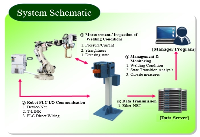
The performance of the proposed method was verified through simulation results using data obtained from the AWIS (Auto Welder Inspection System) welding equipment inspection system as shown in Figs. 1 and 2. The data sets were used for the input value of the multi-layer neural network models.

Fig. 1.

AWIS schematic

Fig. 2.

AWIS operation process

Ⅱ. Proposed fault diagnosis method

2.1 Multi-layer neural network model-based monitoring system

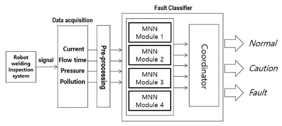
As shown in Fig. 3, the proposed robot welding gun monitoring system uses the amount of current, pressure, flow time, and pollution by the welding equipment inspection apparatus as the input of each multi-layer neural network (MNN) model modules. The failure diagnosis is performed by measuring the progress of aging of the welding gun and output in five states: normal, caution (lower limit), caution (upper limit), warning (lower limit), and warning (upper limit). The coordinator changes the state of the upper and lower limit to one state when the result of the module is caution (upper-lower limit) and fault (upper-lower limit). In other words, if the result of the module is fault (upper-lower limit), the output state is fault. When the result of the module is normal, the output state is normal.

Fig. 3.

Proposed robot welding gun monitoring system

2.2 Multi-layer neural network model

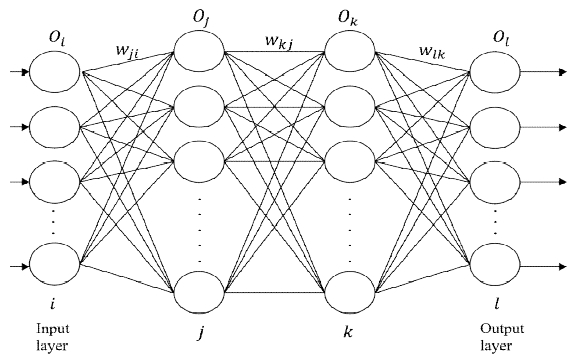
The multi-layer perceptron model implemented in this study is shown in Fig. 4. The cross-entropy model, which is one of the loss function methods, is used to verify the classification performance of the model. The definition of the cross-entropy error is given by equation (1).

Fig. 4.

Structure of the deep multi-layer neural network model

$\[ Crossentropy=-\sum t_l\log \left(\widehat{o_l}\right) \]$

(1)

where, t_l is given as a one-hot vector as the label value. $$ \widehat{o}$$ is the output value of the layer. The cross entropy is used as the loss function in the equation of D_i(t) in Eq. (2) and (3).

Optimization is the process of finding a parameter that minimizes the value of the loss function. In this work, the weight update process is performed using the RMSprop optimization function.

RMSprop is a gradient-based optimization algorithm that takes a moving average into exponentially decreasing weights of previous step gradient squares and computes the learning rate to be inversely proportional to the square root of this value. This is shown in equations (2) and (3) [19][20].

$\[ S_i\left(t\right)=\beta S_i\left(t-1\right)+\left(1-\beta \right)D_i{\left(t\right)}^2 \]$

(2)

$\[ △w_i\left(t\right)=\frac{-\eta }{\sqrt{s_i\left(t\right)+ϵ}}{D}_i{\left(t\right)}^2 \]$

(3)

where β is the decaying factor and η is the learning rate. S_i(t) is the present gradient and is calculated as the exponential average sum of past gradient and gradient variations. D_i(t) is $$ \frac{\partial Loss\left(w_i\left(t\right)\right)}{\partial w_i\left(t\right)}$$. In the MNN model, the neuron adds the bias to the weighted sum of the input and weight values and then determines the output value by the activation function.

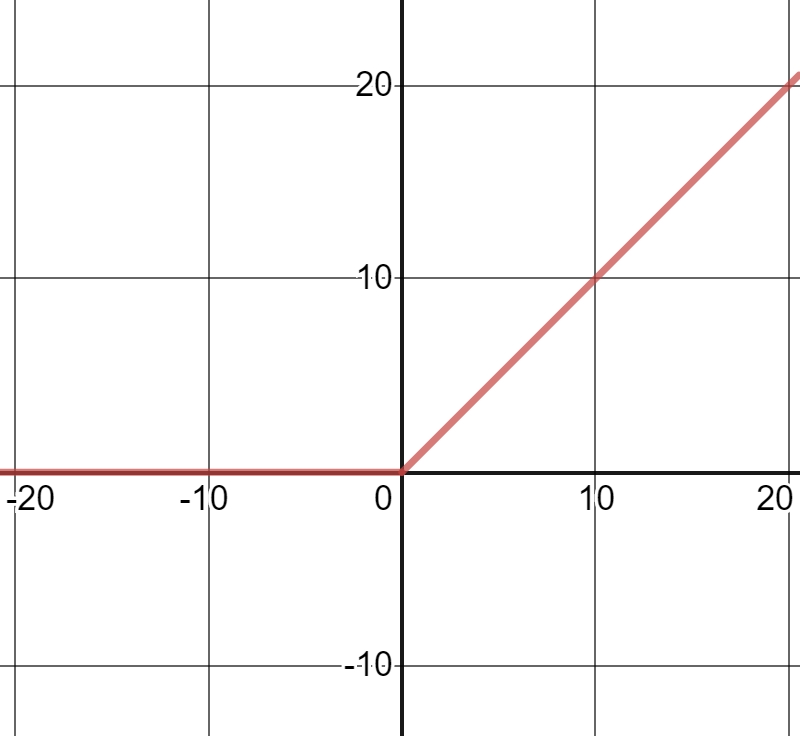
The rectified linear unit ReLU function, which is the most frequently used activation function, is used for the two hidden layers. The ReLU function enables simple calculation of the derivative and has the advantage of fast learning speed. The ReLU function is shown in equation (4)[21].

(4)

where o_n is the output value of the n-th node. The graph of equation (4) is shown in Fig 5.

Fig. 5.

Graph of ReLU function

The Softmax function is used for the output layer. Softmax is used to transform the class classification problem, that is, the output from the previous layer, into the probability of each state when solving the state classification problem. The exponent (exp) is taken for each output and divided by the normalization constant so that the sum is 1. as shown in equation (5) and (6)[22][23].

$\[ a=\sum _j{w}_{ji}{x}_j \]$

(5)

$\[ Softmax\left(a_l\right)=\frac{\mathrm{e}\mathrm{x}\mathrm{p}\left(a_l\right)}{\sum _{i=1}^n\mathrm{e}\mathrm{x}\mathrm{p}\left(a_i\right)} \]$

(6)

In equation (5), a is the output value that is input from the node of the previous layer to the node of the next layer. i is the index of the node of the previous layer, and j is the index of the node of the next layer. In equation (6), n is the output layer of node. and a_i and a_l are the input value input to nodes of the i and l-th output layers, respectively.

Ⅲ. Simulation and results

The simulation environment was implemented using Python 3.5 and the Keras library on Linux OS. The MNN model used in the experiment consists of an input layer, two hidden layers, and an output layer. The input layer consists of 10 nodes, the two hidden layers consist of 32 nodes, and the output layer consists of 5 nodes. However, the module with input of pollution consists of 3 nodes as the output layer. The reason for this is that the current, pressure and flow time are diagnosed in 5 states, pollution is diagnosed in 3 states. The activation function ReLU was used for optimization in the two hidden layers. The learning rate used in learning was 0.001 and the decaying factor was 0.9.

The inputs were simulated by using the amount of current, pressure, flow time, and pollution obtained from the test equipment as inputs to MNN modules 1, 2, 3, and 4, respectively. The training data used in the simulation included the amount of current, pressure, flow time, and pollution. Each dataset consists of 10 samples. In the learning stage, the data of 40 dataset were used for the current, pressure, and flow time. Whereas the pollution was used 24 dataset.

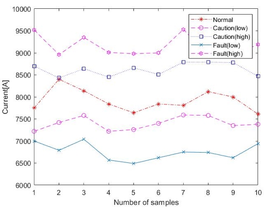
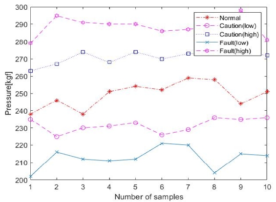
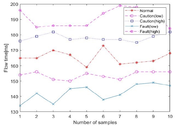
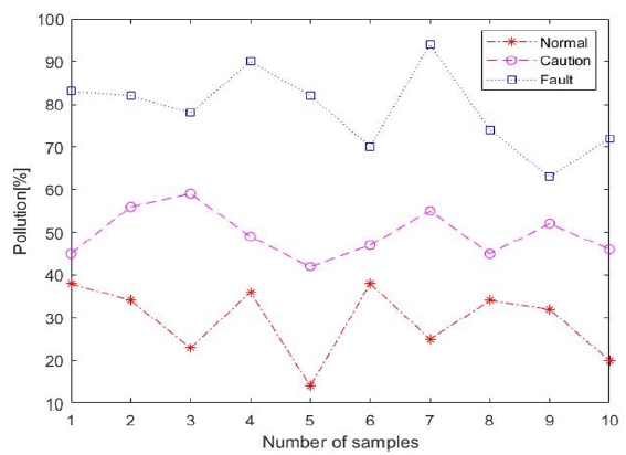
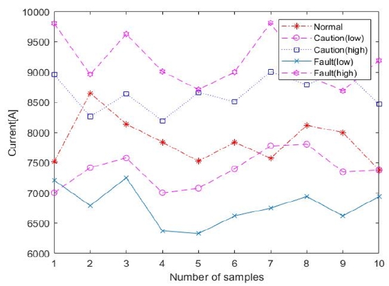
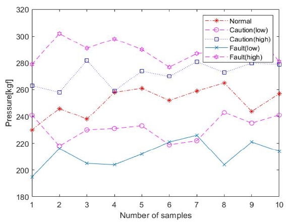
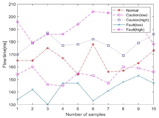
In Figs. 6-8, the test data of current, pressure and flow time were tested with normal, caution (lower limit), caution (upper limit), fault (lower limit), and fault (upper limit) state. In Fig. 9, the test data of the pollution were tested with normal, caution, and fault state.

Fig. 6.

Current test data

Fig. 7.

Pressure test data

Fig. 8.

Flow time test data

Fig. 9.

Pollution test data

Tables 1–4 show the test results for the test data. When generating the result from the module, if the result of the module is normal in the coordinator, the output is the normal state, the output state is Caution for results caution (lower limit) and caution (upper limit), and Fault for results fault (lower limit) and fault (upper limit). Because there are only 3 pollution states, the result of the module in the coordinator becomes the output of the coordinator as is.

Table 1.

Current classification results

Table 2.

Pressure classification results

Table 3.

Flow time classification results

Table 4.

Pollution classification results

The results of the determination of the state of the welding gun show that all the test data exhibited high accuracy and that the state value of the welding gun was accurately determined even at the output part of the coordinator.

Figs. 10–12 show test data randomly considering a noise value of 1~3% in the dataset of the previous Figs. 6–8. Because the dataset of the pollution is not considerably influenced by noise, the dataset of the pollution was not used in this simulation.

Fig. 10.

Current test data considering noise

Fig. 11.

Pressure test data considering noise

Fig. 12.

Flow time test data considering noise

The simulation were carried out under the same state except for noise. The results of the simulation are shown in Tables 5–7.

Table 5.

Classification results at the current test data

Table 6.

Classification results at the pressure test data considering noise

Table 7.

Classification results at the flow time test data considering noise

Simulation results show that the test dataset not considering noise yield approximately 1% to 5% more accurate results than the test dataset considering noise. However, the accuracy is still high for the noisy test dataset. It can be seen that the pressure and the flow time have little influence on the accuracy of discrimination between the test data considering noise and test data not considering noise. Therefore, even if noise is generated in the measured data, the monitoring system will be able to accurately determine the state of the welding gun.

Ⅳ. Conclusions

In this paper, we propose an aging monitoring and fault diagnosis system for robot welding guns using an MNN model. In the proposed method, the failure diagnosis of the robot welding gun was performed using the data obtained from the inspection apparatus as the input values of the multi-layer neural network models. Simulation results show that it is possible to determine the state with high accuracy from the data of current, pressure, flow time, and pollution from the inspection apparatus in the welding gun. It was confirmed that the data of current, pressure, flow time, and pollution in consideration of noise can be discriminated without any problem.

It is expected that the proposed monitoring system will be useful for maintenance of equipment because it can predict the failure of a welding gun by verifying and supplementing the performance through the application in a production line.

References

• I. S. Lee, M. H. Jeong, K. H. Kim, and S. Y. Ha, "Development of an Aging Monitoring System for Robotic Welding Gun using ART2 Neural Networks", Proceedings of KIIT Summer Conference, p158-161, Jun. 2016.
• J. Wagner, and R. Shoureshi, "A Failure Isolation Strategy for Thermofluid System Diagnostics", ASME J. Eng. for Industry, 115(4), p459-465, Nov), (1993. [https://doi.org/10.1115/1.2901790]
• J. Schurmann, "Pattern classification, a unified view of statistical and neural approaches", John Wiley and Sons, New York, (1996).
• J. F. Durodola, N. Li, S. Ramachandra, and A. N. Thite, "A pattern recognition artificial neural network method for random fatigue loading life prediction", International Journal of Fatigue, 99, Part 1 p55-67, Jun), (2017. [https://doi.org/10.1016/j.ijfatigue.2017.02.003]
• F. Xie, H. Fan, Y. Li, Z. Jiang, R. Meng, and A. Bovik, "Melanoma Classification on Dermoscopy Images Using a Neural Network Ensemble Model", IEEE Transactions on Medical Imaging, 36(3), p849-858, Mar), (2017. [https://doi.org/10.1109/tmi.2016.2633551]
• J. Y. Chang, B. J. Lee, S. J. Cho, D. H. Han, and K. H. Lee, "Automatic Classification of Advertising Restaurant Blogs Using Machine Learning Techniques", Journal of IIBC, 16(2), p55-62, Apr), (2016. [https://doi.org/10.7236/jiibc.2016.16.2.55]
• M. S. Kang, Y. G. Jung, and D. H. Jang, "A Study on the Search of Optimal Aquaculture farm condition based on Machine Learning", Journal of IIBC, 17(2), p135-140, Apr), (2017. [https://doi.org/10.7236/jiibc.2017.17.2.135]
• Y. Jiu, L. Wang, Y. Wang, and T. Guo, "A novel memristive Hopfield neural network with application in associative memory", Neurocomputing, 227, p142-148, Mar), (2017.
• F. Wang, C. Yuanlong, and L. Meichun, "pth moment exponential stability of stochastic memristor-basedbidirectional associative memory (BAM) neural networks with timedelays", Neural Networks, 98, p192-202, Feb), (2018. [https://doi.org/10.1016/j.neunet.2017.11.007]
• T. Kohonen, "Self-organizing maps", Springer, Berlin, (1997).
• L. Fausett, "Fundamental of neural netwroks", Prentice Hall, (1994).
• Timmermans, A.J.M, and A.A hulzebosch, "Computer vision system for on-line sorting of pot plants using an artificial neural network classifier", Computer and Electronics in Agriculture, 15(1), p41-55, May), (1996. [https://doi.org/10.1016/0168-1699(95)00056-9]
• R. Isermann, "Process Fault Detection Based on Modeling and Estimation Methods-a Survey", Automatica, 20(4), p387-404, Jul), (1984. [https://doi.org/10.1016/0005-1098(84)90098-0]
• M. M. Polycarpou, and A. T. Vemuri, "Learning Methodology for Failure Detection and Accommodation", IEEE control systems, 15(3), p16-24, Jun), (1995.
• T. Sorsa, H. N. Koivo, and H. Koivisto, "Neural Networks in Process Fault Diagnosis", IEEE transactions on systems, man and cybernetics, 21(4), p815-825, Jul/Aug), (1991.
• M. A. Kramer, and J. A. Leonard, "Diagnosis Using Back Propagation Neural Networks Analysis and Criticism", Computers & Chemical Engineering, 14(12), p1323-1338, Dec), (1990. [https://doi.org/10.1016/0098-1354(90)80015-4]
• I. S. Lee, J. T. Kim, J. W. Lee, Y. J. Lee, and K. Y. Kim, "Neural Networks-Based Fault Detection and Isolation of Nonlinear Systems", IASTED International Conference on Neural Networks and Computational Intelligence, Cancun, Mexico, p142-147, May. 2003.
• I. S. Lee, and G. Lee, "Fault Detection and Isolation Using Artificial Neural Networks", Proc. of the ISCA Int’l Conference on Computer Applications in Industry and Engineering, p335-340, Jun. 2006.
• S. M. Ahn, Y. J. Chung, J. J. Lee, and J. H. Yang, "Korean Sentence Generation Using Phoneme-Level LSTM Language Model", Journal of Intelligent Information Systems website, 23(2), p71-88, Jun), (2017.
• http://www.cs.toronto.edu/~tijmen/csc321/slides/lecture_slides_lec6.pdf, [accessed: Oct. 02, 2018]
• Nair, V Hinton, and G. E. Hinton, "Rectified linear units improve restricted boltzmann machines", In Proceedings of the 27th international conference on machine learning (ICML-10), Haifa, Israel, p807-814, Jun. 2010.
• S. Gold, and A. Rangarajan, "Softmax to softassign: Neural network algorithms for combinatorial optimization", Journal of Artificial Neural Networks, p381-399, (1996).
• M. W. Mak, "Lecture Notes on Backpropagation", Technical Report and Lecture Note Series, Department of Electronic and Information Engineering, The Hong Kong Polytechnic University, Jul), (2015.